Enter the Big Data Matrix: analyzing meanings and relations of everything (2/2)
Running the Python example step by step:
We explained the basic idea behind LSA or latent semantic analysis in the first part of this blog.
- We built a matrix by word counting for each document. The set of document vectors are then sorted by words they appear in.
- Then we applied SVD (single value decomposition) on the document and took a smaller number of Eigen values to shrink the three newly decomposed matrices. We keep these three smaller matrices as the basis for our data model.
- Any new documents can be computed by a formula rather than having to run SVD again.
- We can then use the new matrix to compute the similarities of word vectors.
In the second part of this tutorial, we’ll go through a simple example with real code.
This is the original corpus.
Word count gives us a matrix composed by Matrix[ row of words, column document]
Compute SVD using NumPy
Let’s run the actual code, you can find the Python code here in github. A matlab script is also available.
First, start the PyLab console Window. If you have not downloaded Enthought Python Distribution, please get it from the download link.
from numpy import *
from numpy.linalg import svd
The SVD solver is part of the NumPy package.
The next step is to enter the word matrix that represent all the sentences and word occurrences in them.
A = array ([( 1., 0., 0., 1., 0., 0., 0., 0., 0.),
( 1., 0., 1., 0., 0., 0., 0., 0., 0.),
( 1., 1., 0., 0., 0., 0., 0., 0., 0.),
( 0., 1., 1., 0., 1., 0., 0., 0., 0.),
( 0., 1., 1., 2., 0., 0., 0., 0., 0.),
( 0., 1., 0., 0., 1., 0., 0., 0., 0.),
( 0., 1., 0., 0., 1., 0., 0., 0., 0.),
( 0., 0., 1., 1., 0., 0., 0., 0., 0.),
( 0., 1., 0., 0., 0., 0., 0., 0., 1.),
( 0., 0., 0., 0., 0., 1., 1., 1., 0.),
( 0., 0., 0., 0., 0., 0., 1., 1., 1.),
( 0., 0., 0., 0., 0., 0., 0., 1., 1.)])
Now run apply SVD to decompose the matrix into 3:
U,sigma,V = svd(A) // Numpy built in function.
Results of the decomposition, you get 3 Matrices, U, sigma (W Matrix), V. Let me explain each one of them.
The U Matrix
These values are basically a coefficient times the original vector, you are looking at the U matrix.
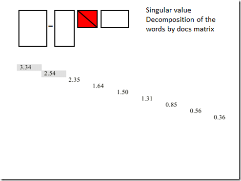
The sigma Matrix (W matrix)
Or the one that contains all the Eigen values on its diagonal, we will be pick to use perhaps 2 of these Eigen values for our work. Why 2? That is purely by experimentation. In general you should pick about 300 in a really large matrix, and 2-3 in a really small matrix like this one. Your job as the data scientist is to play with the model and find the optimal number of Eigen value for this particular dataset.
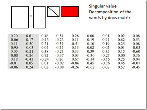
The V Transposed Matrix
This is the word matrix, or the Vt matrix.
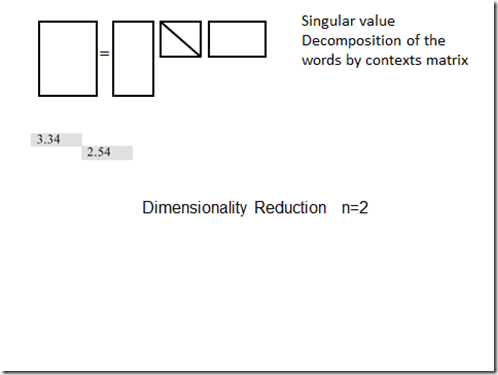
Dimension Reduction
As discussed earlier, the next step is to do a dimension reduction. In our case, we pick n=2. We are trying to compute the 3 new matrices in this step. U matrix should have 2 columns, W(Sigma) matrix should have 2x2, and the Vt matrix should have 2 rows.
In the code, we will make a new matrix and copy over 2 Eigen values.
Sigma = zeros_like(A) # A temp matrix A filled with 0. Same as Sigma = A.copy().fill(0)

n = min(A.shape) # should return 9, since the original A matrix is 12 x 9, the shorter dimension is 9 which is N.
Sigma[:n,:n] = diag(sigma) # Fill the matrix with Eigen values in diagonal.
U2=U[:,:2] take 2 columns of the decomposed U matrix.
S2=Sigma[:2,:2] ## take 2 Eigen values for the new W Matrix. (N xN) in the middle.
V=transpose(V)
V2=V[:,:2] # take two rows of V(transposed); The matrix to the right.
Multiply them back,
A2=dot(U2,dot(S2,transpose(V2))
The New Matrix ready for computing meaning of words
This is the New Matrix that we now can use to compute the relations. Notice we are comparing the word vectors using the Cosine function.
print "relation between human and user: ", dot(A2[0,:],A2[ 3,:])/linalg.norm(A2[0,:])/linalg.norm(A2[ 3,:]) # human is close to user (row 0, row 3)
print "relation between human and minor: ", dot(A2[0,:],A2[11,:])/linalg.norm(A2[0,:])/linalg.norm(A2[11,:]) #minors in this context has nothing to do with human. (row 0, row 11)
Human and minor = similar at 0.8878; human minors = –0.275 (not similar).
print "relation between tree and graph: ", dot(A2[9,:],A2[10,:])/linalg.norm(A2[9,:])/linalg.norm(A2[10,:]) #(row 9, row 10)
Conclusion
This example shows you how advanced math models can be applied to text to figure out the relations between words. The same technique can be applied to just about anything that can be turned into a feature vector. Data scientists can fine tune these models to discover interesting things, and ask new questions that normal BI can not help answer. SVD is very useful in big data computation and predictive analysis, you will encounter it often in data analysis.
Questions or comments? follow me on twitter @wenmingye


