Data Science Toolkit - Logistic regression models
To support our client's ability to predict user response to their digital advertising Xandr provides custom models based on decision trees. We developed an easy-to-use programming language called Bonsai that enables users to create decision trees to dynamically populate line item parameters.
Decision trees work well for simple discrete models that map into traditional targeting-based forms of prediction but struggle to effectively model what amounts to a sparse matrix of many dimensions and large categorical features. Bonsai is easy to understand and easy to use but not always sufficient for machines and data scientists as it doesn't allow the efficient representation of the relationships between features. For these more complex needs, Xandr uses logistic regression models.
Logistic regression is the basic approach to predict the probability of a binary response (click or don't click; buy or don't buy) from a combination of multiple signals. By utilizing logistic regression data scientists can run more expressive models that produce more accurate predictions and that can be quickly trained at a high scale. By building tailored algorithms, clients with sophisticated data science tools can achieve better performance than the built-in optimization provided by Xandr and can run complex offline models in real-time.
Formula for logistic regression
Logistic regression is a classification algorithm. It is used to predict a binary outcome (such as will click, will not click) based on a set of independent variables.
The formula for logistic regression is:
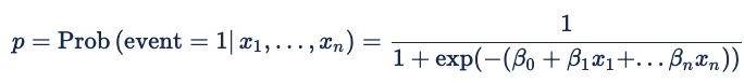
Where the probability (p) being modeled is that of a binary outcome: event = 1 or event = 0. For online advertising, the event is a click, a pixel fire, or another online action. The probability is conditional on both the predictors x1 through xn and on an implicit set of variables that represent the features in a bid request. The beta coefficients are the weights that the model assigns to the different predictors.
We convert this probability of an event happening to an expected value by multiplying the probability by the event's value (e.g., the eCPC goal for a click prediction), adding an additive offset to the estimate, and then applying min/max expected value limits to reduce the impact of mispredictions.
The formula for deriving an expected value for an impression from the probability of an event happening is:
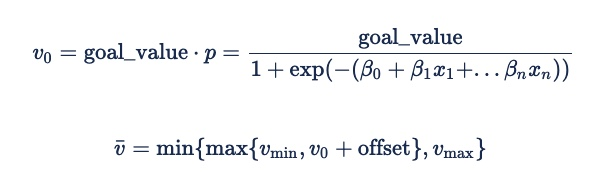
The offset will usually be 0. However, a negative value may be useful as a security factor to ensure performance at the expense of delivery on low-performing inventory. That will ensure that the advertiser does not bid instead of bidding very little and potentially incurring fixed fees.
Example using categorical features from online advertising
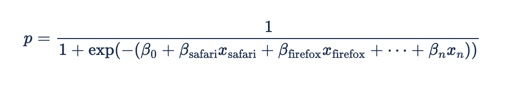
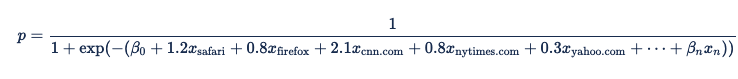
Online advertising has many categorical features, that is, features that can have many possible values. Some examples include browser, domain, and day of the week. These features are usually represented with "one-hot" encoding (using "dummy variables"), meaning that x1 would be 1 if "browser = safari" and 0 if not, x2 would be 1 if "browser = firefox", and so on.
If we put this into the logistic regression formula, we get:
Since browser is a categorical feature, we can express the coefficients in a table:
| Browser | Coefficient |
|---|---|
| safari | 1.2 |
| firefox | 0.8 |
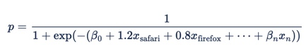
Each row of this table is converted to a term in the logistic regression formula, so x1 = 1 if "browser = safari" and β safari = 1.2 and x2 = 1 if "browser = firefox" and β firefox = 0.8. This makes the overall equation:
Other categorical features can be expressed this way as well. Suppose we assigned the following values as coefficients to the following domains:
| Domain | Coefficient |
|---|---|
| cnn.com | 2.1 |
| nytimes.com | 0.8 |
| yahoo.com | 0.3 |
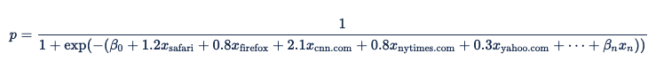
These values then become incremental terms in the formula (x3 is 1 if "domain = cnn.com" and β 3 is 2.1), making the overall equation:
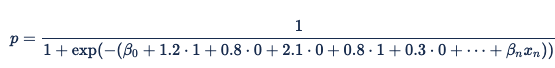
When the ad impression is served, Xandr identifies the browser as Safari and the domain as nytimes.com. The corresponding variables for browser = Safari and domain = nytimes.com are set to 1 and the other variables are set to 0, resulting in the equation:
Higher-order predictors
Xandr supports higher-order predictors (combinations of features), allowing custom models to handle complex interactions between predictors. Start with the previous example calculating a value based on the categorical values of domain and browser. Now imagine that domain and browser are not independent and that you need to model the relationship between them. To do this, you can create a two-way categorical feature with a coefficient for each pair of features, using the values specified in the table below:
| Browser | Domain | Coefficient |
|---|---|---|
| Safari | cnn.com | 1.1 |
| Safari | nytimes.com | 1.3 |
| Safari | yahoo.com | 1.2 |
| Firefox | cnn.com | 3.3 |
| Firefox | nytimes.com | 0.7 |
| Firefox | yahoo.com | 0.1 |
Each of these paired predictors becomes a term in the logistic regression equation:

Hashed predictors
Combining multiple categorical predictors creates extremely large tables that cannot be easily mapped into memory for a real-time system. Instead of trying to pull values from such tables, you can hash the feature combinations to create collisions – in effect, reducing the number of combinations that need to be mapped into memory in real-time.
Example of hashed predictors
As a simple example, you can hash the browser-domain combinations from the previous example using a 2-bit hash function:
| Browser | Domain | Coefficient |
|---|---|---|
| Safari | cnn.com | 0 |
| Safari | nytimes.com | 1 |
| Safari | yahoo.com | 3 |
| Firefox | cnn.com | 2 |
| Firefox | nytimes.com | 0 |
| Firefox | yahoo.com | 1 |
Then compute a coefficient for each hash value. Note that there are fewer features than in the previous example, potentially capturing some of the cross-feature interaction without requiring as much memory.
| Browser-Domain Hash | Coefficient |
|---|---|
| 0 | 1.3 |
| 1 | 0.7 |
| 2 | 1.5 |
| 3 | 0.9 |
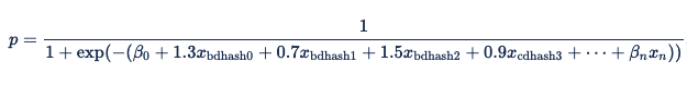
Once you replace the variables with these values, the logistic regression equation becomes:
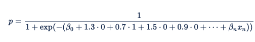
To predict the response on a particular impression, Xandr hashes the detected features (using the same hash function that is applied during feature engineering for both training the models and online inference). For some features, we use hash functions to hash the raw feature values to the ones used in the above formula and executes the prediction. If the browser is Safari and the domain is nytimes.com (or any other browser-domain pair that hashes to the same value), we hash these to find the value 1 and substitute that into the logistic regression equation:
Conversion from one-hot encoded and weight vectors to tables
The encoding for categorical features ensures that, for each categorical feature, at most one variable will receive the value 1 and everything else will receive a value of zero. The dot product of the browser features' weight and the browser variables is thus a roundabout way to activate the predetermined weight for the browser on the bid request. The Digital Platform API uses the below equation, which is a standard Sigmoid function:

If we had the following ad request:
If the browser type is Firefox then with one-hot encoding x_firefox would be set to 1 and x_safari would be set to 0. The activated weight for the Firefox type would be its predetermined weight of 0.8 multiplied by the encoded value of 1. So x_firefox would equal 0.8. The activated weight for the Safari type would be 0, it's predetermined weight, 1.2 multiplied by the x_safari setting of 0.
We would get an equation with the following weighting:
In order to define the mapping from categorical feature to weight, Xandr uses API calls to create and update lookup tables. The logistic regression model itself will refer to these tables and not to a vector of one-hot encoded variables. The model may also directly refer to cardinal or real values, including segment age, segment value, and frequency or recency information for an advertiser, a creative, or a line item.
Sample process overview
Let's use the information from above to create a sample workflow.
Suppose you set up an exploratory campaign to gather training data with a small budget. You wish to optimize a given retargeting line item to minimize cost-per-click. Each impression won generates a row in the Log Level Data Feeds with the is_click column set to false. When a click is eventually generated, an identical row is generated in the data feed with the is_click column set to true. You partition the data between the training, validation, and testing sets by looking at the last few bits of user_id_64. The user_id_64 determines which part the data will be assigned to. You eventually determine that the key variables are:
- The user's browser (categorical)
- The user's country and day of the week (higher-order categorical)
- The combination of the publisher and the user's country (higher-order categorical)
- The amount of time since an ad for that advertiser was last showed to that user (advertiser recency, a cardinal value)
Since there aren't that many browsers, it's reasonable to have one weight for each browser in your training set. The cross-product and country and day of the week is also reasonably small. The combination of publisher and country, however, has a high cardinality, so you arbitrarily decide to train that with a hashed table of 4096 entries. Finally, the line item's daily frequency is a cardinal value.
For each row in LLD, you first filter out rows that do not come from your training campaign. Now that you have defined the events you're interested in, you can extract the variables:
- browser ID
- country ID
- user's day of the week (by adding the timezone offset to the impression's timestamp and mapping that to a 7-day week)
- publisher ID
- advertiser recency, with a max of one hour (if this is the first ad we're showing to this user, the recency defaults to one hour)
You reserve one feature ID for recency and 4096 IDs for the hashed (publisher:country), and dynamically generate feature IDs for each browser and (country:day of week) pair. The hashed feature needs one more extra step: you take the two IDs (publisher and country), write them out to a little endian vector of 8 32-bit integers, and find the bucket with MurmurHash3_x86_32(vector, 32, 0xC0FFEE) % 4096 (0xC0FFEE is an arbitrary seed). That gives you a (sparse) vector of feature values for each row, so you can count the number of impressions and the number of clicks for each such vector.
After a day of slowly buying impressions, you try the logistic regression model you trained on (a subset of) LLD. The sparse vector of feature values is a one-hot encoding of the feature space. You must convert back from this encoding to the more logical functions from categorical value to weight (lookup tables). To do this join the table of feature to feature ID and the vector of weights to get the following:
| Feature | Index | Weight |
|---|---|---|
| Advertiser recency | 0 | -0.2 |
| publisher:country-bucket 0 | 1 | 1.4 |
| publisher:country-bucket 1 | 2 | -2.1 |
| ... | ... | ... |
| publisher:country-bucket 4095 | 4096 | -0.5 |
| browser=safari | 4097 | 5.2 |
| country:day-of-week=US:monday | 4098 | 0.7 |
| ... | ... | ... |
You determine the weights for each feature:
- Advertiser-recency: You read the weight directly from the trained model.
- The hashed table: You read the weights for the 4096 features and put them in an array.
- Browser: You walk the dynamic map from feature to ID, the features are the keys and the ID the values, and build a lookup table from browser ID to non-zero weight (with zero as the default) to create a list of browser to weight mappings.
- Country:day of week: You walk the dynamic map from feature to ID and build a lookup table from browser ID to non-zero weight (with zero as the default) to create a list of browser to weight mappings.
This is all the data you need to call the AppNexus API.
Overview of auction time process
Once the line item passes targeting, Xandr uses its logistic regression model to determine a bid price:
- For each lookup table in its description, Xandr extracts the field's (or fields') value(s) from the bid request, and looks for an entry in the table. If there is an entry, that value is added to the linear argument of the logistic function. Otherwise, the table's default value, which is usually 0, is used.
- The same is done for hashed tables, except that Xandr hashes the values to find a bucket, and then look for that bucket in the hashed table's list of bucket -> value mappings. Again, the default value is used if the specified value does not appear in the table.
- Finally, Xandr looks for Bonsai features. We perform the lookup for each feature, multiply by the weight, and apply min/max limits.
- Xandr then sums the components and Beta0 and passes that to the logistic function to compute the estimated probability of a click. The estimated probability is multiplied by the goal value to obtain the expected value, which is then clamped between 1 and 100 CPM to curb any unrealistically high valuations.
- Xandr then uses the expected value and the amount of inventory available to compute a bid. The exact computations vary depending on the line item's setup, but the result is that Xandr will automatically scale down the expected value until the bids are just high enough that the line item spends its daily budget at the end of each day. For more information on this scaling, see Adaptive Pacing (log in required) in documentation.