Building an Azure Analysis Services Model on Top of Azure Blob Storage—Part 2
The first part in this series covering Azure Analysis Services models on top of Azure Blob Storage discussed techniques to implement a small Tabular 1400 model based on synthetic TPC-DS source data. This second part continues the journey to take Tabular 1400 in Azure Analysis Services to larger scale factors—up to the maximum capacity that Azure Analysis Services currently provides.
Taking a Tabular 1400 model to large scale requires an efficient approach that mitigates limitations in the tools and maximizes performance in the model. For starters, it would take a long time to generate 1 TB of TPC-DS source data by using a single dsdgen instance. A much better approach is to run multiple dsdgen instances in parallel to save time and create a 1 TB set of smaller source files that are easier to handle individually. Furthermore, having generated and uploaded the source data to Azure Blob storage, it would not be advisable to create the Tabular model directly against the full set of data because SQL Server Data Tools for Analysis Services Tabular (SSDT Tabular) would attempt to download all that data to the workspace server. Even if the workspace server had the capacity, it’s an unnecessarily large data transfer. Instead, it is a common best practice to create a representative subset of the data and then build the data model against that source, and then later switch the source during production deployment. Moreover, the Tabular 1400 model must be designed with data management and performance requirements in mind. Among other things, this includes a partitioning scheme for the tables in the model. And last but not least, the source queries of the table partitions should be optimized to avoid redundancies and keep the model metadata clean and small. The May 2017 release of SSDT Tabular introduces support for named expressions in Tabular 1400 models and this article demonstrates how to use them for source query optimization.
Generating 1 TB of TPC-DS source data by using multiple dsdgen instances is easy thanks to the command line parameters PARALLEL and CHILD. The PARALLEL parameter indicates the overall number of child processes to generate the source data. The CHILD parameter defines which particular chunk of data a particular dsdgen instance generates. For example, I distributed the data generation across 10 virtual machines in Azure, with each VM running 10 child dsdgen instances. Running in parallel, these 10 instances utilized the eight available cores per VM close to 100% and finished the data generation in roughly 2 hours. The following screenshot shows the resource utilization on one of the VMs about half an hour into the processing. 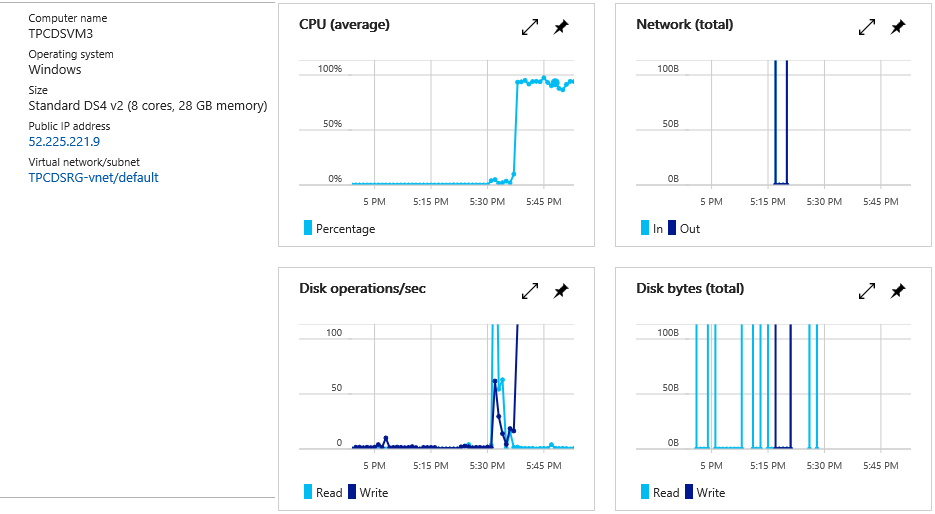
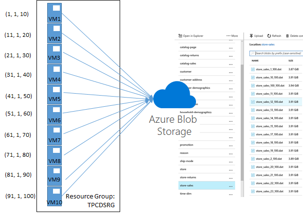
Windows PowerShell and the Azure Resource Manager cmdlets make provisioning 10 Azure VMs a blast. For a sample script to create a fully configured virtual machine, see the article “Create a fully configured virtual machine with PowerShell.” I then installed AzCopy via https://aka.ms/downloadazcopypr and copied the TPC-DS tool set and an empty data folder with all the sub-containers to each VM (as discussed in Part 1). Next, I slightly modified the batch file from Part 1 to create and upload the source files to accommodate the different file name format that dsdgen uses when PARALLEL and CHILD parameters are specified. Instead of <table name>.dat, dsdgen now generates files names as <table name>_<child id>_<parallel total>.dat. An additional batch file then helped to launch the 10 data generation processes, passing in the child ID and Blob service endpoint URL as parameters. It’s a trivial batch as listed below. On the second VM, the loop would start at 11 and go to 20, and so forth (see the following illustration).
@echo off
for /l %%x in (1, 1, 10) do (
start createandupload.bat %%x https:// <BlobStorageAccount> .blob.core.windows.net/
)
Having finished the data generation and verified that all files were uploaded to Azure Blob storage successfully, I deleted all provisioned VM resources by using a single Remove-AzureRmResourceGroup command. Deleting a resource group deletes all associated Azure resources. Needless to say that the Azure Blob storage account with the generated data must not be associated with this resource group for it must remain available for the next steps.
The next task is to create a representative sample of the TPC-DS data for modelling purposes. This can be as easy as placing the 1 GB data set generated in Part 1 in a separate Azure Blob storage account. However, dsdgen creates a different set of source files per table for the 1 GB versus the 1 TB scale factor, even if the same PARALLEL and CHILD parameters are specified. If it is important to generate the same set of source files just with less data—and in my case it is because I want to create source queries on top of a large collection of blobs representative of a 1 TB data set—a different approach is needed.
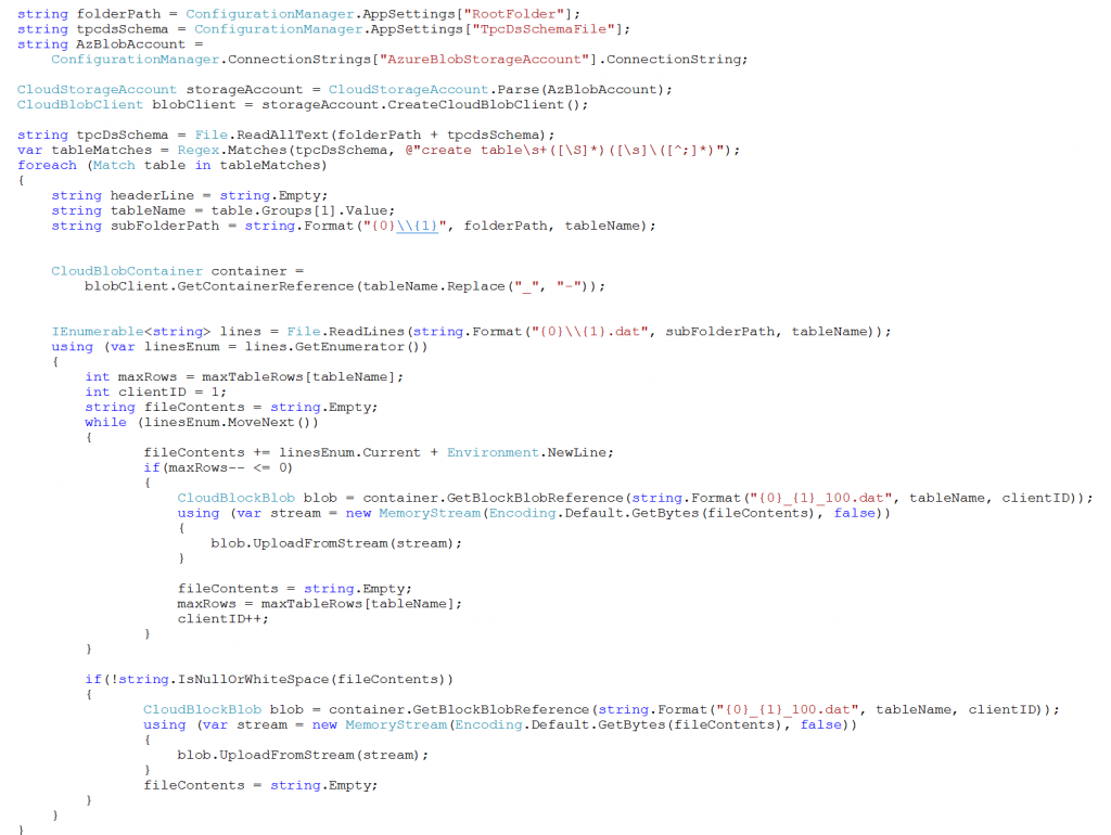
By using the 1 GB data set from Part 1 and the code snippet below, I generated a representative set of sample files identical to the ones that dsdgen generates for a 1 TB data set. The following table summarizes how the code snippet distributed the 1 GB of data across the sample files. The code snippet then used the Azure SDK to upload the files to my second Azure Blob storage account.
| Table Name | Row Count (1GB) | File Count (1TB) | Max Rows Per Sample File |
| call_center | 6 | 1 | 6 |
| catalog_page | 11718 | 1 | 11718 |
| catalog_returns | 144067 | 100 | 1441 |
| catalog_sales | 1441548 | 100 | 14416 |
| customer | 100000 | 100 | 1000 |
| customer_address | 50000 | 100 | 500 |
| customer_demographics | 1920800 | 100 | 19208 |
| date_dim | 73049 | 1 | 73049 |
| dbgen_version | 1 | 1 | 1 |
| household_demographics | 7200 | 1 | 7200 |
| income_band | 20 | 1 | 20 |
| inventory | 11745000 | 100 | 117450 |
| item | 18000 | 1 | 18000 |
| promotion | 300 | 1 | 300 |
| reason | 35 | 1 | 35 |
| ship_mode | 20 | 1 | 20 |
| store | 12 | 1 | 12 |
| store_returns | 287514 | 100 | 2876 |
| store_sales | 2880404 | 100 | 28805 |
| time_dim | 86400 | 1 | 86400 |
| warehouse | 5 | 1 | 5 |
| web_page | 60 | 1 | 60 |
| web_returns | 71763 | 100 | 718 |
| web_sales | 719384 | 100 | 7194 |
| web_site | 30 | 1 | 30 |
The code is not very efficient, but it does get the job done eventually—giving me enough time to think about the partitioning scheme for the larger tables in the model. If you study the available Performance Guide for Analysis Services Tabular, you will find that the partitioning of tables in a Tabular model does not help to improve query performance. However, starting with SQL Server 2016 Analysis Services, Tabular models can process multiple partitions in parallel, so partitioning can help to improve processing performance. Still, as the performance guide points out, excessive partitioning could result in many small column segments, which could impact query performance. It’s therefore best to be conservative. A main reason for partitioning in Tabular models is to aid in incremental data loading, which is precisely my intention.
The goal is to load as much TPC-DS data as possible into a Tabular 1400 model. The largest Azure Analysis Services server currently has 20 cores and 100 GB of RAM. Even larger servers with 200 GB or 400 GB of RAM will be available soon. So, how large of a Tabular 1400 model can such a server load? The answer depends on, among other things, the compressibility of the source data. Achievable ratios can vary widely. With a cautious assumption of 2:1 compressibility, 1 TB of source data would far exceed 100 GB of RAM. It’s going to be necessary to start with smaller subsets. And even if a larger server could fit all the source data into 400 GB of RAM, it would still be advisable to go for incremental data loading. The data set consists of more than 1,000 blob files. Pulling all these files into a Tabular model at once would likely hit throttling thresholds on the Azure Blob storage side causing substantial delays during processing.
The TPC-DS tables can be categorized as follows:
| Category | Tables | Amount of Data |
| Small tables with only 1 source file per table. | call_center, catalog_page, date_dim, dbgen_version, household_demographics, income_band, item, promotion, reason, ship_mode, store, time_dim, warehouse, web_page, web_site | ~0.1 GB |
| Medium tables with 100 source files per table. | customer, customer_address,customer_demographics | ~5 GB |
| Large tables with 100 source files per table. | catalog_returns, catalog_sales, inventory, store_returns, store_sales, web_returns, web_sales | ~950 GB |
The small tables with only 1 source file per table can be imported at once. These tables do not require an incremental loading strategy. Similarly, the medium files do not add much data and can be loaded in full, but the large tables require a staged approach. So, the first processing cycle will include all files for the small and medium tables, but only the first source file for each large table. This reduces the source data volume to approximately 10 GB for the initial processing cycle. Subsequent processing cycles can then add further partitions to the large tables to import the remaining data until RAM capacity is exhausted on the Azure Analysis Services server. The following diagram illustrates this staged loading process. 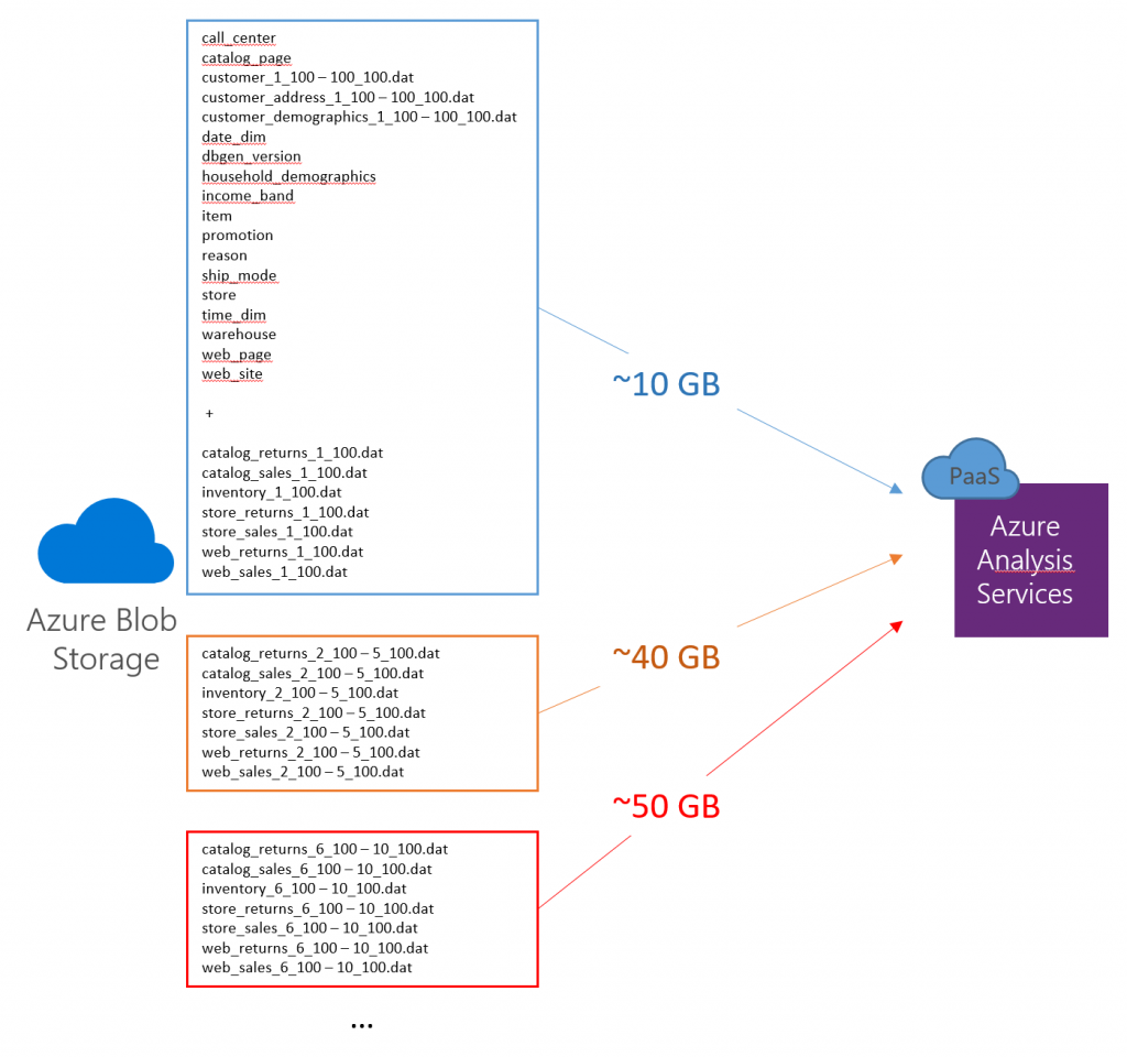
By using the 1 GB sample data set in Azure Blob storage, I can now build a Tabular 1400 model by using the May 2017 release of SSDT Tabular and implement the staged loading process by taking advantage of named expressions in the source queries. Note that previous SSDT Tabular releases are not able to deal with named expressions. The May (or a later) release is an absolute must have.
Regarding source queries, the small tables with a single source file don’t require any special attention. The source queries covered in Part 1 would suffice. So, let’s take one of the more interesting medium tables that comprises 100 source files, such as the customer table, create the source query for that table, and then see how the result could apply in a similar way to all other tables in the model.
The first step is to create a source query for the customer table by using Query Builder in SSDT Tabular. And the first task is to exclude the header file from the list of data files. It will be included later. In Navigator, select the customer table, and then in Query Builder, right-click on the Name cell in the last row (showing a value of “header_customer.dat”), expand Text Filters, and then select Does not start with. Next, in the Applied Steps list, for the resulting Filtered Rows step, click on the Settings button, and then in the Filter Rows dialog box, change the value for "does not begin with" from "header_customer.dat" to just "header" so that this filter can be applied later on in the same way to any header file in the data set. Click OK and verify that the header file has disappeared from the list of source files.
The next task is to combine the remaining files for the table. In the header cell of the Content column, click on the Combine Files button, as illustrated in the following screenshot, and then in the Combine Files dialog box, click OK. 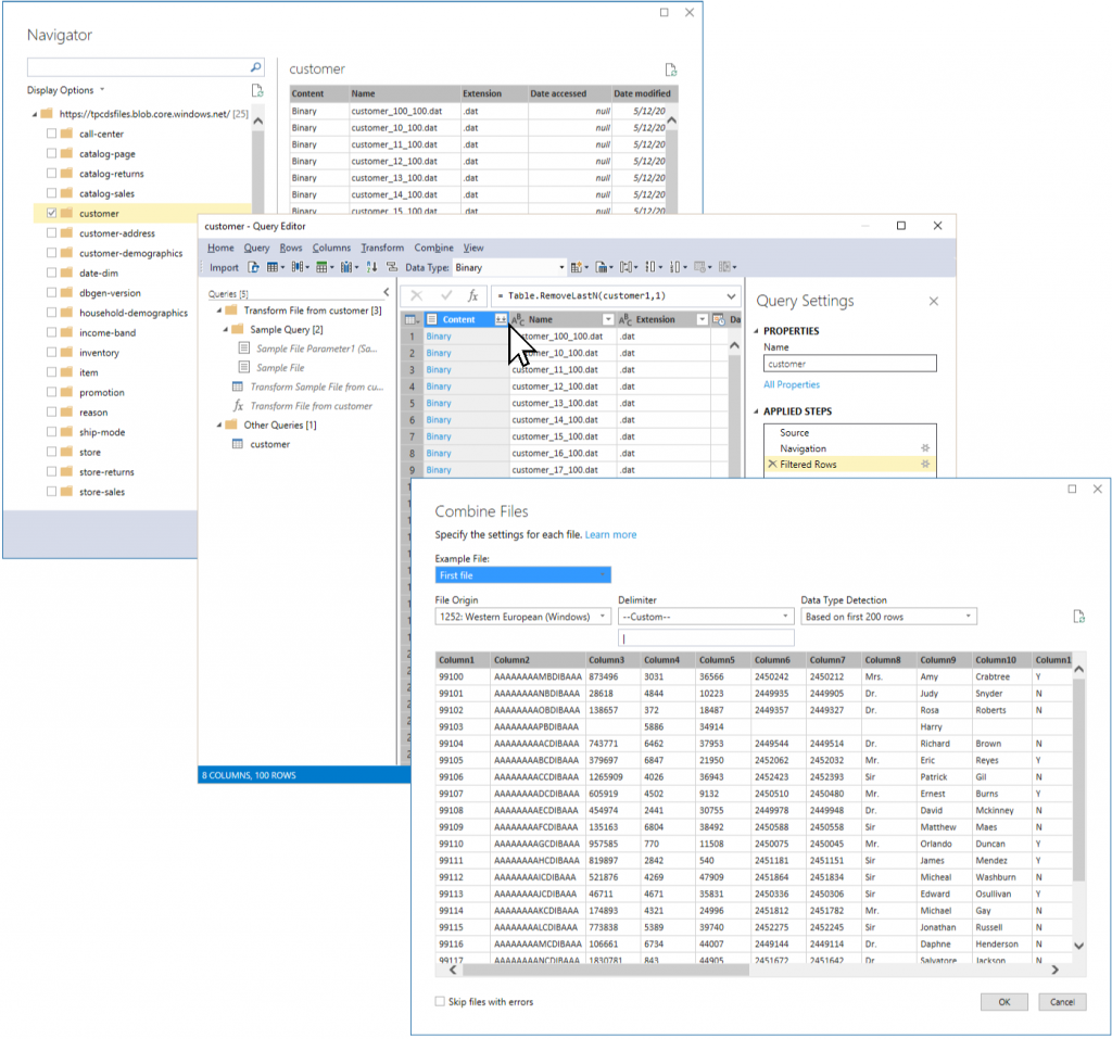
As you can see in the Queries pane above, this sequence of steps creates quite a few new expressions, which the customer query relies on to combine the 100 source files for the table. However, apart from the fact that the header file still needs to be added to get the column names, it is a good idea to optimize the expressions at this point to keep the model free of clutter. The sample queries are unnecessary and should be eliminated. This is especially notable when importing many tables. In the TPC-DS case with 25 tables, Query Builder would generate 25 different sets of these sample queries, which would amount to a total of 75 avoidable expressions in the model. The only named expression worth keeping is the Transform File from customer function. Again, Query Builder would generate multiple such transform functions (one for each table) where only a single such function suffices.
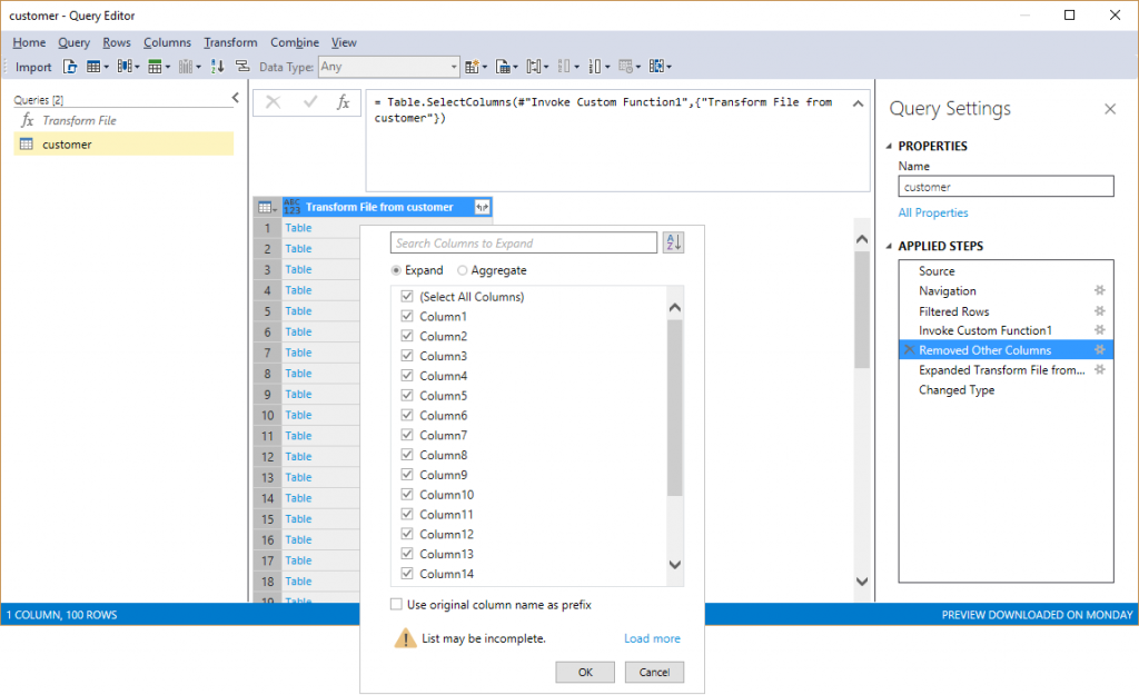
The first cleanup step is to eliminate the need for the sample queries by editing the customer source query. In Query Builder, in the Applied Steps list, delete all steps after the “Invoke Custom Function 1” step so that this invoke step is the last step in the query, which adds a “Transform File from customer” column to the table. Right-click this column and select Remove other Columns so that it is the only remaining column. Next, click on the Expand button in this column’s header, and then make sure you deselect the Use original column name as prefix checkbox and click OK. At this point, the customer query no longer references any sample expressions so they can be deleted in Query Builder. Also, rename the “Transform File from customer” function and just call it “Transform File” as in the screenshot below so that it can be used across multiple tables without causing confusion. I also shortened the M expression for this function as follows.
let
Source = (File) => let
Source = Csv.Document(File,[Delimiter="|"])
in
Source
in
Source
Note that even the Transform File function could be eliminated by replacing its reference in the Invoke Custom Function1 step with a direct call to the Csv.Document function, as in each Csv.Document([Content],[Delimiter="|"]) . But don’t eliminate the Transform File function just yet.
The next task is to extend the customer query to discover and apply the header file dynamically. This involves the following high-level steps:
| Step | M Expression |
| Get all files from the Blob container for the customer table that start with “header”. | #"Get Header File List" = Table.SelectRows(customer1, each Text.StartsWith([Name], "header")) |
| Read the content of the first file from this list by using the Transform File function. There should only be one header file. Any additional files would be ignored. | #"Read First Header File" = #"Transform File"(#"Get Header File List"{0}[Content]), |
| Transform the first row from this header file into a table. | #"Headers Table" = Record.ToTable(#"Read First Header File"{0}) |
| Clean up the headers table by removing any rows that have no values. | #"Cleaned Headers Table" = Table.SelectRows(#"Headers Table", each [Value] <> null and [Value] <> "") |
| Modify the Expanded Transform File step and replace the long lists of static column references with the Name and Value lists from the cleaned headers table. | #"Expanded Transform File" = Table.ExpandTableColumn(#"Removed Other Columns", "Transform File", #"Cleaned Headers Table"[Name], #"Cleaned Headers Table"[Value]) |
The result is a customer table that includes all source files from the table’s Blob container with the correct header names, as in the following screenshot. 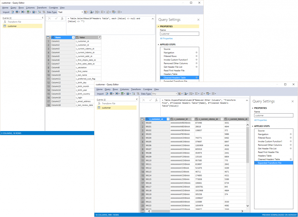
This is great progress, but the job is not yet done. The next challenge is to convert this source query into a global function so that it can be used across all tables, not just the customer table. The existing Transform File function can serve as a template for the new function. In Query Builder, right-click on Transform File, and select Duplicate. Give the new function a meaningful name, such as ReadBlobData.
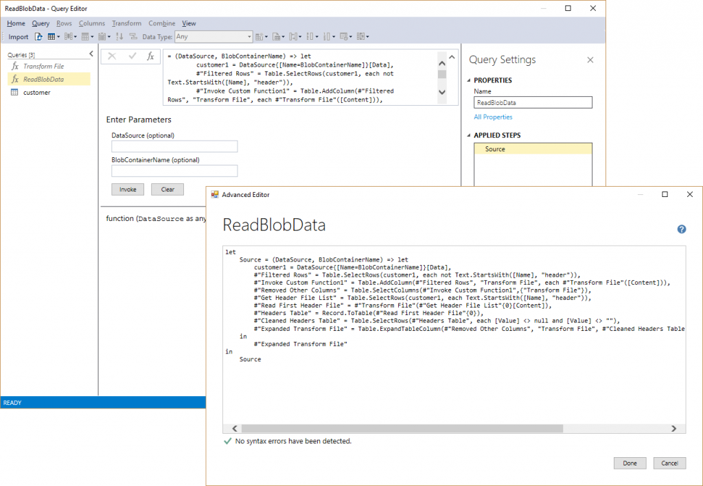
M functions follow the format = (Parameter List) => let statement. As parameters, I use DataSource and BlobContainerName, and the let statement is almost an exact copy of the query for the customer table, except that I replaced the data source and container references with the corresponding DataSource and BlobContainerName parameters. It’s relatively straightforward to copy and adjust the entire source query by using Advanced Editor, as in the screenshot below. Also, make sure to save the original source query in a separate text file because it might be needed again. The next step then is to replace the customer source query and call the ReadBlobData function instead, as follows (note that the data source name is specific to my data model):
let
Source = #"AzureBlobs/https://tpcdsfiles blob core windows net/",
BlobData = ReadBlobData(Source, "customer")
in
BlobData
The results so far suffice for the customer table, but there is one more requirement to support the staged imports for the large tables. In other words, the ReadBlobData function should not just read all the source files from a given Azure Blob container at once but in specified ranges. In Query Editor, this is easy to add to the original table query. It is not so easy to do in a complex named expression, such as the ReadBlobData function. Unfortunately, editing a complex named expression in Query Editor almost always requires jumping into the Advanced Editor. No doubt, there is room for improvements in future SSDT Tabular releases.
As workaround, I temporarily reverted the customer query using my previously saved copy, selected the Filtered Rows step, and then on the Rows menu, selected Keep Range of Rows. After clicking Insert in the Insert Step dialog box, I specified appropriate values for the First row and Number of rows parameters and clicked OK (see the following screenshot). 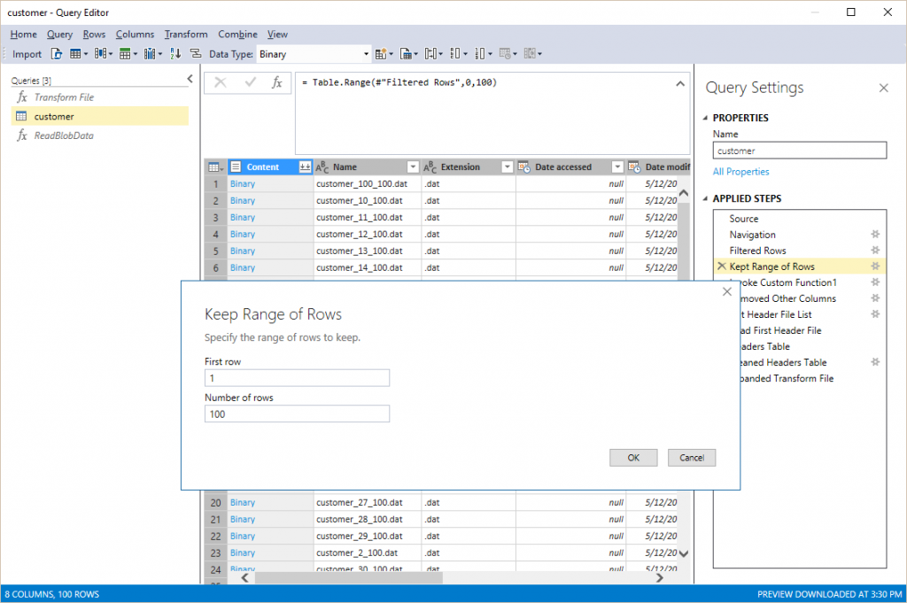
The new Kept Range of Rows step then needed to be inserted into the ReadBlobData function in between the Filtered Rows and the Invoke Custom Function1 steps in Advanced Editor. The ReadBlobData function also required two additional parameters called FirstRow and NumberOfRows, as in #"Kept Range of Rows" = Table.Range(#"Filtered Rows", Value.Subtract(FirstRow, 1),NumberOfRows) . Note that the Query Builder UI considers the value of 1 to refer to row 0, so the ReadBlobData function uses the Value.Substract function to maintain this behavior for the FirstRow parameter. This completes the ReadBlobData function (see the following code listing). It can now be called from all source queries in the model, as summarized in the table below.
let
Source = (DataSource, BlobContainerName, FirstRow, NumberOfRows) => let
customer1 = DataSource{[Name=BlobContainerName]}[Data],
#"Filtered Rows" = Table.SelectRows(customer1, each not Text.StartsWith([Name], "header")),
#"Kept Range of Rows" = Table.Range(#"Filtered Rows",Value.Subtract(FirstRow, 1),NumberOfRows),
#"Invoke Custom Function1" = Table.AddColumn(#"Kept Range of Rows", "Transform File", each #"Transform File"([Content])),
#"Removed Other Columns" = Table.SelectColumns(#"Invoke Custom Function1",{"Transform File"}),
#"Get Header File List" = Table.SelectRows(customer1, each Text.StartsWith([Name], "header")),
#"Read First Header File" = #"Transform File"(#"Get Header File List"{0}[Content]),
#"Headers Table" = Record.ToTable(#"Read First Header File"{0}),
#"Cleaned Headers Table" = Table.SelectRows(#"Headers Table", each [Value] <> null and [Value] <> ""),
#"Expanded Transform File" = Table.ExpandTableColumn(#"Removed Other Columns", "Transform File", #"Cleaned Headers Table"[Name], #"Cleaned Headers Table"[Value])
in
#"Expanded Transform File"
in
Source
| Category | Source Query |
| Small tables with only 1 source file per table. | letSource = #"AzureBlobs/https://tpcdsfiles blob core windows net/",BlobData = ReadBlobData(Source, "<blob container name>", 1, 1)inBlobData |
| Medium tables with 100 source files per table. | letSource = #"AzureBlobs/https://tpcdsfiles blob core windows net/",BlobData = ReadBlobData(Source, "<blob container name>", 1, 100)inBlobData |
| Large tables with 100 source files per table. | letSource = #"AzureBlobs/https://tpcdsfiles blob core windows net/",BlobData = ReadBlobData(Source, "<blob container name>", 1, 1)inBlobData |
It is straightforward to create the 25 TPC-DS tables in the model by using the above source query pattern. Still, there is one more issue that must be addressed and that is that the source queries do not yet detect the data types for the table columns. This is an important prerequisite to analyzing the data. For each table, I modified the source query as follows:
- In Query Builder on the Rows menu, select all columns.
- On the Transform menu, under Any Column, select Detect Data Type.
- Display Advanced Editor and double-check that the detected data type for each column in the Changed Type step is correct.
As a side note, instead of editing the source query of an existing table, it is currently better to delete the table and recreate it from scratch. There are still some work items left to finish before the table editing in SSDT Tabular can work reliably.
And that’s it as far as creating the tables for my TPC-DS Tabular 1400 model is concerned. The initial data load into the workspace model finishes quickly because I’m working against the 1 GB sample data set. The row counts in the following screenshot confirm that only a small subset of the data is imported. 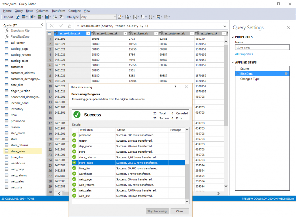
The Tabular model is now ready for deployment to an Azure Analysis Services server. Apart from updating the deployment settings in the Tabular project properties to point SSDT Tabular to the desired target server, this would require changing the data source definition to import the data from the actual 1 TB data set. In Tabular Model Explorer, this can be accomplished by right-clicking on the existing data source object, and then choosing Change Source, which displays the Azure Blob Storage dialog box to update the Account name or URL, as in the following screenshot. 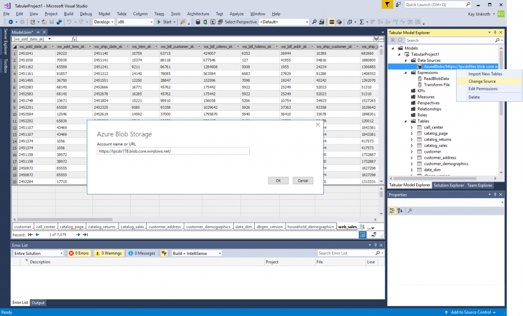
Finally, the model can be deployed by switching to Solution Explorer, right-clicking on the project node, and selecting Deploy. If necessary, SSDT will prompt for the access key before deploying the model. Processing only takes minutes because the source queries only import a few gigabytes at this time (see the screenshots below for processor activity and memory consumption on the Azure Analysis Server during and after processing). Having finished the deployment and initial processing, it is a good idea to change the data source definition again to revert to the 1 GB sample data set. This helps to avoid accidentally downloading large amounts of data to the SSDT workstation. 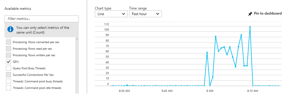

And that’s it for this round of working with a Tabular 1400 model in Azure Analysis Services on top of Azure Blob storage. The data model is now deployed. The next part is to add partitions to load more data. For this part, I am going to switch from SSDT Tabular to SQL Server Management Studio (SSMS), Tabular Model Scripting Language (TMSL), and Tabular Object Model (TOM) in Azure Functions. One of the main reasons is that SSDT Tabular does not facilitate incremental modifications to a model. It prefers to deploy models in an all or nothing method, which is not suitable for the data load strategy discussed in the current article. SSMS, TMSL, and TOM provide finer control. So, stay tuned for part 3 in this series to put Azure Analysis Services under some serious data pressure.
And as always, please take Tabular 1400 for a test drive. Send us your feedback and suggestions by using ProBIToolsFeedback or SSASPrev at Microsoft.com. Or use any other available communication channels such as UserVoice or MSDN forums. Influence the evolution of the Analysis Services connectivity stack to the benefit of all our customers!
Comments
- Anonymous
June 01, 2017
Great articles mate, keep it up!
